Coursera Capstone: Text Analysis

Unnest

Now we have our data in a tidy format, we really need to unpack the lines so we can analyze word counts. To do this, tidytext::unnest_tokens() comes in very handy.

At the same time I am going to handle the unknown encoding of the corpus, with a regular expression designed to only allow lower case letters A-Z and apostrophes. By default unnest_tokens() converts everything to lower case.

Side Note Unknown encoding of apostrophe’s, caused me serval stressful nights, loosing my mind doing failed equality comparrisons with characters that appeared the same on my screen.

# unnest_tokens as single words
word_sources <- map(tidy_sources, ~ unnest_tokens(., word, text))

# method to catch "foriegn" characters
word_sources %<>% map(~ mutate(., word = str_extract(word, "[a-z]+'?[a-z]+")))

# percent "foriegn" words, NAs now
map(word_sources, ~ sum(is.na(.$word)) / nrow(.))

## $news
## [1] 0.05982832
## 
## $twitter
## [1] 0.06846871
## 
## $blogs
## [1] 0.05923256

# drop NAs
word_sources %<>% map(~ filter(., !is.na(word)))

That is a crude method to determine if a word is from a “foriegn” language, but it is good in the sense it is extremely restictive. That makes doing proper filtering possible in later stage. In a scenario like this where we have an abundance of data, filtering out a corrupted ~ 5% is accetable.

Stop Words

I also also want to drop “stop” words. These are hyper-common words with little to no impact in terms of text analysis. Words like “the”, “of”, and “a” all fall into this category and while these words make up the bulk of our corpus, they hold minimal predictive or sentimental value. I will show the top 20 words before and after removing “stop” words:

# Before
# plot the top 20 raw
plot_df <- word_sources %>%
    map_df(~ count(., word, sort = T) %>%
               top_n(20), .id = "source") %>% 
    mutate(word = reorder(word, n))

## Selecting by n
## Selecting by n
## Selecting by n

ggplot(plot_df, aes(x = word, y = n, fill = source)) +
    geom_col(show.legend = F) +
    coord_flip() +
    facet_wrap(~ source, scales = "free")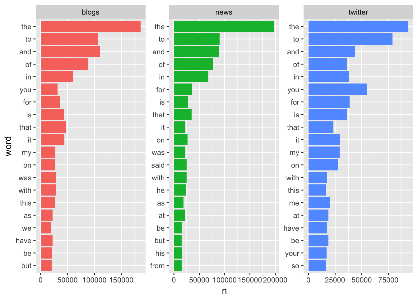

# top 1000 make up 70 %
word_sources %>%
    map_df(~ count(., word, sort = T) %>%
               mutate(rel_freq = n / sum(n)), .id = "source") %>%
    group_by(source) %>%
    top_n(1000) %>%
    summarise(percent_total = sum(rel_freq))

## Selecting by rel_freq

## # A tibble: 3 x 2
##    source percent_total
##     <chr>         <dbl>
## 1   blogs     0.7213822
## 2    news     0.6703697
## 3 twitter     0.7461815

# 3 lexicons built in
data(stop_words)

# clean stop_words just like sourcew above
stop_words %<>% mutate(word = str_extract(word, "[a-z]+'?[a-z]+")) %>%
      filter(!is.na(word))
# add custom "stop" words
stop_words %<>% full_join(tibble(word = c("i", "m", "ve", "t", "don", "can", "st"), lexicon = "cust"))

## Joining, by = c("word", "lexicon")

word_sources %<>% map(~ anti_join(., stop_words))

## Joining, by = "word"

## Joining, by = "word"
## Joining, by = "word"

# After
# now re-plot the top 20
plot_df2 <- word_sources %>%
    map_df(~ count(., word, sort = T) %>%
               top_n(20), .id = "source") %>% 
    mutate(word = reorder(word, n))

## Selecting by n

## Selecting by n
## Selecting by n

ggplot(plot_df2, aes(x = word, y = n, fill = source)) +
    geom_col(show.legend = F) +
    coord_flip() +
    facet_wrap(~ source, scales = "free")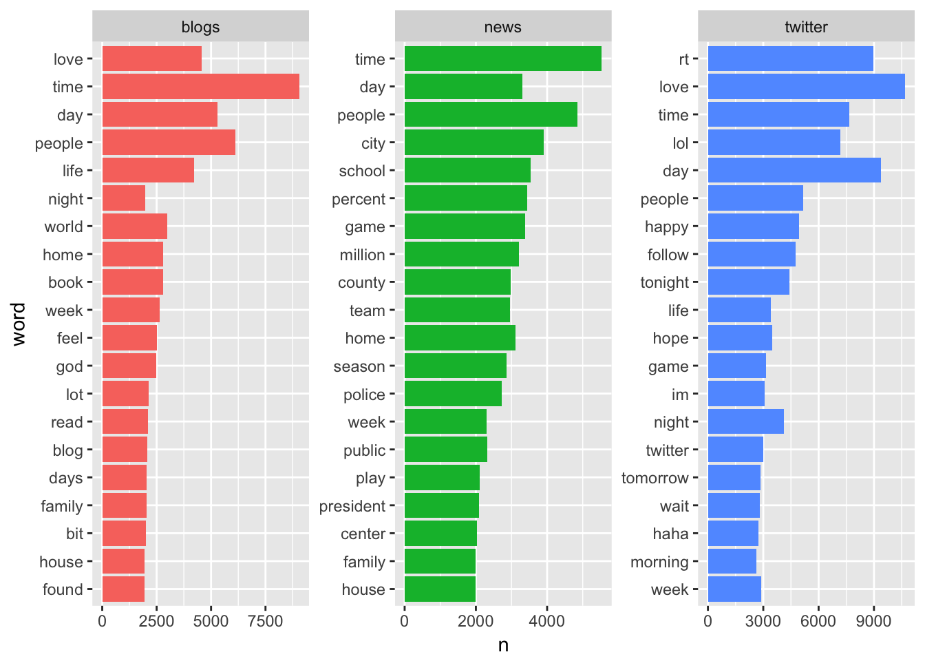

# now top 1000 make up 40-50 %
word_sources %>%
    map_df(~ count(., word, sort = T) %>%
               mutate(rel_freq = n / sum(n)), .id = "source") %>%
    group_by(source) %>%
    top_n(1000) %>%
    summarise(percent_total = sum(rel_freq))

## Selecting by rel_freq

## # A tibble: 3 x 2
##    source percent_total
##     <chr>         <dbl>
## 1   blogs     0.4105591
## 2    news     0.4049446
## 3 twitter     0.5065281

stop_words %<>% full_join(tibble(word = c("rt", "im", "follow"), lexicon = "cust"))

## Joining, by = c("word", "lexicon")

Notice, there are some specific Twitter words, like “rt”, “follow”, and “im”, in the top20 and I’ve added these to the stop_words. I think these words are more about the structure of the community and less about actual communicative text.

Neighborhood

Now we have a dataframe of with counts of bigrams that appear more than 2 times. We can easily turn this into a graph object and plot it to look at patters. For this example I am looking at the first order neighborhood around “fast”:

# make a large network
tnet <- graph_from_data_frame(g2_counts[,1:2])
# weight the edges with count data
E(tnet)$weight <- g2_counts$n

# this is just a short hand reference variable
v <- grep("fast", V(tnet)$name)[1]

# make 1-edge "neighborhood" network of around v
small_net <- make_ego_graph(tnet, order = 1, nodes = v)[[1]]

# plot it
ggraph(small_net, layout = "nicely") + 
    geom_edge_link(aes(width = log(weight),
                       alpha = log(weight)),
                   arrow = arrow(length = unit(10, 'mm')),
                   end_cap = circle(5, 'mm'),
                   edge_colour = "purple",
                   show.legend = F) +
    geom_node_label(aes(label = name),
                    size = 5) +
    scale_edge_alpha(range = c(.1, .9)) +
    theme_void()

We can see a lot of relationship that make sense, like “fast food”, “fast lane” and “move fast”. The edge thickness and transparency are scaled to show the probability of the association and the arrows show direction from first word to second word. It’s always nice to look at the data to make sure things behaving like expected. Note, so of the nodes are connected directly without going through “fast” and this is because we started with a much larger network and are only plotting the “neighborhood” one node away from our target.

Make it fast

Inorder to build something that is quick for look ups we need to perform and store most of these calculations ahead of time. One simple method of doing this would be to build an ordered top 10 (or top ‘n’) list of second words for each first word in our data set (and store it in a big list). Since lots of first words will not have a full 10 associated second words we are going to back-fill the remaining slots with the top 10 words in frequency from the dataset overall. In a real world setting, taking advantage of the ability to record, analyse and update our bigram probabilities based on user history would make this tool much better, but for now this is a quick proof of concept and display of speed.

# if we want to do this fast lets make a list of top10's or topn's
my_n <- 10

# grab the topn for each first word
topn_list <- g2_counts %>%
    split(.$w1) %>%
    map(~ top_n(., my_n)) # these are the trade-offs we make
# looks good, but some groups don't have 10 preditions

# fill these gaps with the top 10 overall words
topn_overall <- count(word_sources[["twitter"]], word, sort = T) %>%
    top_n(my_n) %>%
    select(word) %>%
    unlist()
# long term we could do this within the specific og document (i.e. chapter, post, etc...)

# anon() for map(.f)
anon <- function(df) {
    if (nrow(df) < my_n) {
        df %<>% bind_rows(tibble(w1 = unique(df$w1),
                                 w2 = topn_overall[1:(my_n - nrow(df))],
                                 n = 1) ) }
    return(df) }
# run anon on the list
topn_list %<>% map(anon)

# lets ungroup and lean it out
topn_lean <- map(topn_list, ~ ungroup(.) %>%
                     select(pred = w2, n) %>%
                     mutate(p = n / sum(n)))

topn_lean[["fast"]] # with probabilities

## # A tibble: 10 x 3
##           pred     n          p
##          <chr> <dbl>      <dbl>
##  1        food    20 0.28169014
##  2     forward    18 0.25352113
##  3 approaching     9 0.12676056
##  4       paced     7 0.09859155
##  5        lane     4 0.05633803
##  6       break     3 0.04225352
##  7         lol     3 0.04225352
##  8        time     3 0.04225352
##  9       track     3 0.04225352
## 10        love     1 0.01408451

system.time( topn_lean[["fast"]] ) # wow that's fast

##    user  system elapsed 
##       0       0       0