State Park Popularity
2017/05/17
 .
.
This project is from the UVA UseR Meetup on May 17, 2017. This meetup was hack-a-thon-ish, with the goal of quickly constructing some exploratory analysis.
In this analysis I use library(ggmap) to utilize Google’s awesome map tools within the familiar framework of R’s library(ggplot2). My goal is to overlay public data about visitor volume to see just where people like to get outside and enjoy nature in the good ol’ USA.
Globals
I am a huge believer in the library(tidyverse) and this project would not have been possible without the great library(ggmaps) that makes working with Google Maps way too easy.
knitr::opts_chunk$set(echo = TRUE, message = FALSE)
library(ggmap)
library(cowplot)
library(viridis) # pretty colors
library(tidyverse)
library(magrittr) # for `%<>%`
Read in
#  2016 data from: https://irma.nps.gov/Stats/SSRSReports/National%20Reports/Annual%20Park%20Ranking%20Report%20(1979%20-%20Last%20Calendar%20Year)
datf <- read.csv("~/Downloads/Annual Park Ranking Report %281979 - Last Calendar Year%29.csv")[-(1:2),] %>%
    rownames_to_column(var = "park")
geo-code it
Nothing to see here but the workhorse, ggmap::geo_code(), which will interpret a wide range of character inputs into latitude and longitude coordinates. I really like the magrittr::%<>%, because I feel it makes most common data cleaning steps type easier.
# Guess lat-lon via ggmaps::geo_codes()
# message: this takes a while, you are limited to 2000 queries per day on Google
geo_codes <- geocode(datf$park) # so save it separate for safety
datf %<>% bind_cols(geo_codes)
## Clean for plotting scales
datf$Bookmark %<>% gsub("\\%", "", .) %>% # why did they name it "BookMark""
as.numeric()
datf$ParkType %<>% gsub(",", "", .) %>% as.numeric()Plot on a map
Just using the Google Maps API to select a base layer so we can initialize a ggplot graphic with a latitude and longitude grid where we can overlay our geo coded National Parks data.
# get map object from Google API
usa <-get_map(location='united states', zoom=4)

# Use map layer as base layer
ggmap(usa, "device") + # then resume normal geoms on a lat lon coord system
    geom_point(data = datf, aes(lon, lat, size = ParkType, fill = log10(ParkType)),
               alpha = .5, shape = 21, show.legend = F) +
    scale_size_continuous(range = c(1,15)) +
    scale_fill_viridis()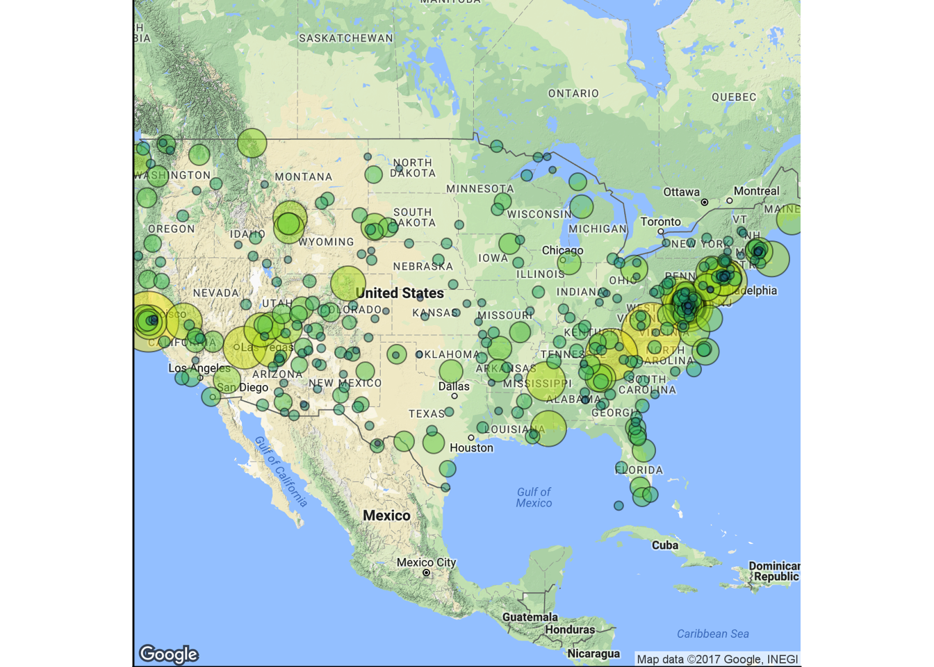
That’s a lot of parks along the East Coast, which you’d expect with the dense coastal population and the Appalachian Mountains running from Georgia to Maine. Looks like the most visited parks seem to cluster around the San Francisco, California and Washington DC.
cp <- list()

# DC
dc <- get_map(location = "charlottesville va", zoom = 7)
cp[[1]] <- ggmap(dc, "device") +
    geom_point(data = datf, aes(lon, lat, size = ParkType, fill = log10(ParkType)),
               alpha = .5, shape = 21, show.legend = F) +
    scale_size_continuous(range = c(1,15)) +
    scale_fill_viridis()

# Cali
ca <- get_map(location = "sacramento ca", zoom = 7)
cp[[2]] <- ggmap(ca, "device") +
    geom_point(data = datf, aes(lon, lat, size = ParkType, fill = log10(ParkType)),
               alpha = .5, shape = 21, show.legend = F) +
    scale_size_continuous(range = c(1,15)) +
    scale_fill_viridis()

plot_grid(cp[[1]], cp[[2]])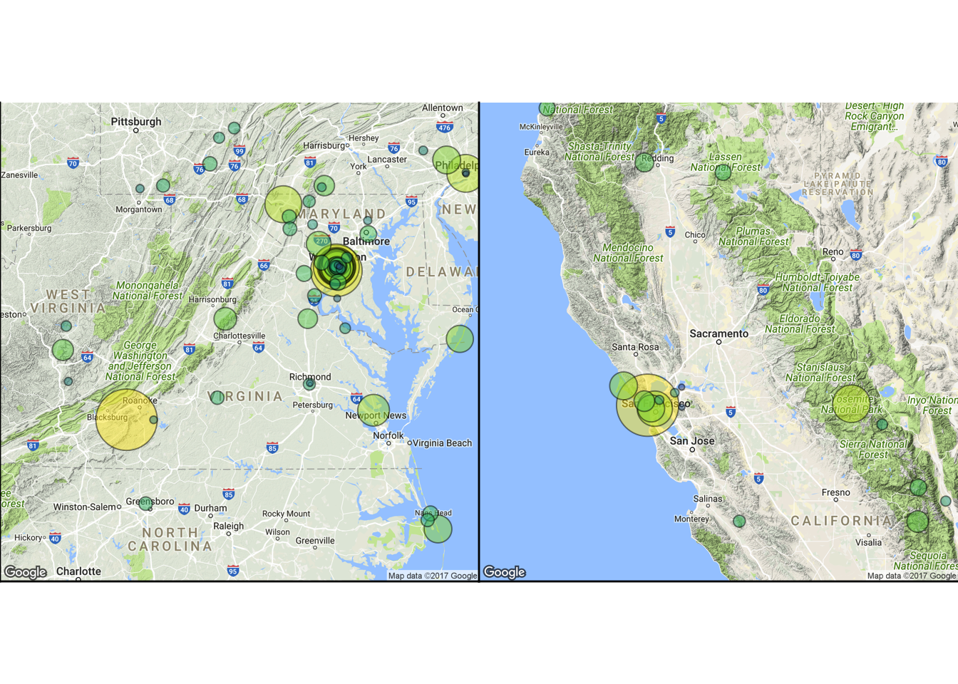
Wrap up
I can highly recommend that big yellow dot in South West Virginia, it’s the Blue Ridge Parkway! Maybe I’m biased because I live in Charllottesville, but the Blue Ridge Parkway way stretches all the way along the mountains in Virginia, making for super scenic drives and overlooks. With its easy access and proximity to Washington DC, no wonder it is one of the most popular parks in the whole country.
Thanks for reading, and check out the UVA UseR Group on MeetUp. It’s a great group of really nice and nerdy people that do a bunch of different things with R, plus they usually have free food and give away Amazon gift cards as door prizes!!!
