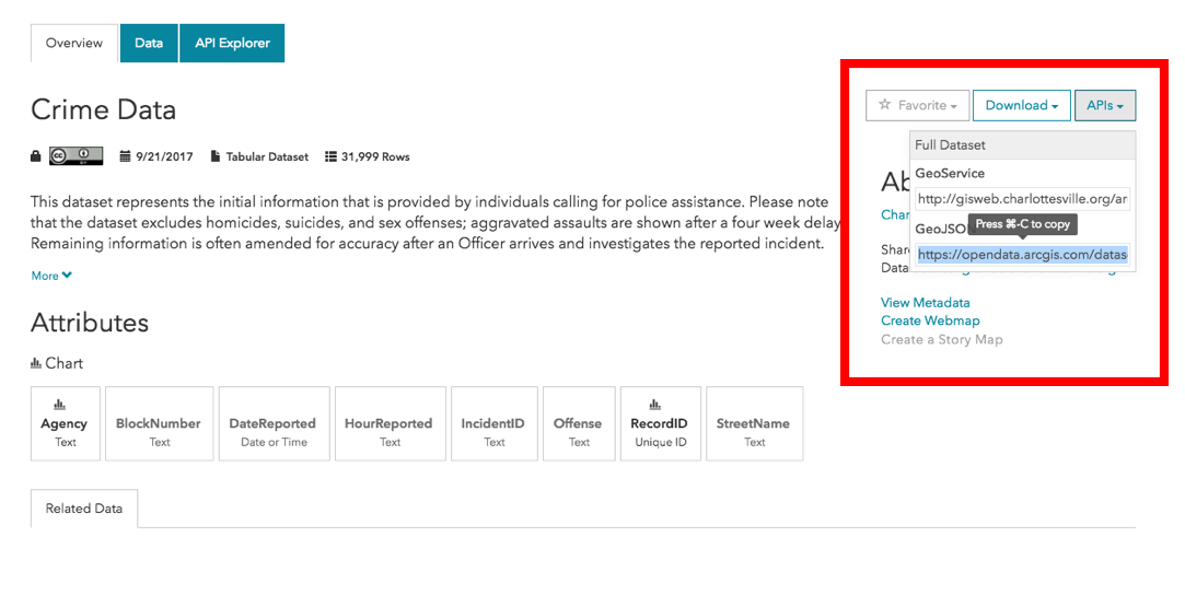
And then let our our new best friend library(geojsonio) do the heavy lifting. The library(geojsonio) is designed to handle geographic data in the GeoJSON and TopoJSON formats. It contains the function geojson_read() for accessing data via url or local file path. We will use it on the link stored in our clipboard.

library(geojsonio) #v_0.4.2
crime_json <- geojson_read("https://opendata.arcgis.com/datasets/d1877e350fad45d192d233d2b2600156_7.geojson",
                           parse = TRUE) # ~1-5 minutes
# parse = TRUE attempts to parse to data.frame like structures; default is FALSE

Our read-in returned a large list (4.3 Mb) with two elements, $type and $features. If you are using RStudio the newest development version (v1.1.379) offers enhanced views for lists and other objects:

View(crime_json) # we could also click on the object in the 'Environment' tab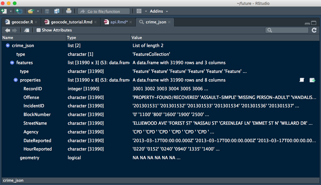

There are some other nice perks in the preview, including an intergrated console and the modern dark theme! You can download the preview here.

The data that we are after is in the second element .$features, but we can see from our View() look-in that it is formatted slightly weird. Let’s look at the top rows:

crime_df <- crime_json[["features"]]
head(crime_df)

##      type properties.RecordID              properties.Offense
## 1 Feature                3001             TRAFFIC-HIT AND RUN
## 2 Feature                3002  BURGLARY/BREAKING AND ENTERING
## 3 Feature                3003                    TRAFFIC STOP
## 4 Feature                3004                  ASSAULT-SIMPLE
## 5 Feature                3005 MOTOR VEHICLE THEFT/STOLEN AUTO
## 6 Feature                3006       TRESPASS ON REAL PROPERTY
##   properties.IncidentID properties.BlockNumber properties.StreetName
## 1             201302116                   1600        UNIVERSITY AVE
## 2             201302117                    300            14TH ST NW
## 3             201302118                    800            CHERRY AVE
## 4             201302119                    100      OLD FIFTH CIRCLE
## 5             201302120                   1500           CARLTON AVE
## 6             201302121                      0            N EMMET ST
##   properties.Agency properties.DateReported properties.HourReported
## 1              CPD   2013/04/15 00:00:00+00                    2345
## 2              CPD   2013/04/16 00:00:00+00                    0010
## 3              CPD   2013/04/16 00:00:00+00                    0032
## 4              CPD   2013/04/16 00:00:00+00                    0732
## 5              CPD   2013/04/16 00:00:00+00                    0720
## 6              CPD   2013/04/16 00:00:00+00                    0925
##   geometry
## 1       NA
## 2       NA
## 3       NA
## 4       NA
## 5       NA
## 6       NA

If you are really paying attention you might realize that the dimensions of crime_df are 32000x3, and the second column properties is a bunch of 8X1 dataframes. head() silently “unnested” properties and printed it as if it were a real 32000x11 dataframe. The last column geometry is all NAs for this data set because it is just a table of text information. In the next section we will see this change when accessing the API for shape files.

All that’s left to do is to extract just the properties column and we will have a nice dataframe ready to start analyzing!

crime_df <-  crime_df[[2]]

With only a couple of lines of code, we have accessed all of the Crime Data released by the Charlottesville Police Department to date on the ODP. This is exactly the same data we would have if we downloaded the ‘csv’ file by hand and read it in using readr::read_csv(), but now we did it all with reproducible code!

If you want to keep going with this data and start cleaning it up for your analysis check out the begining of my towing forcast.

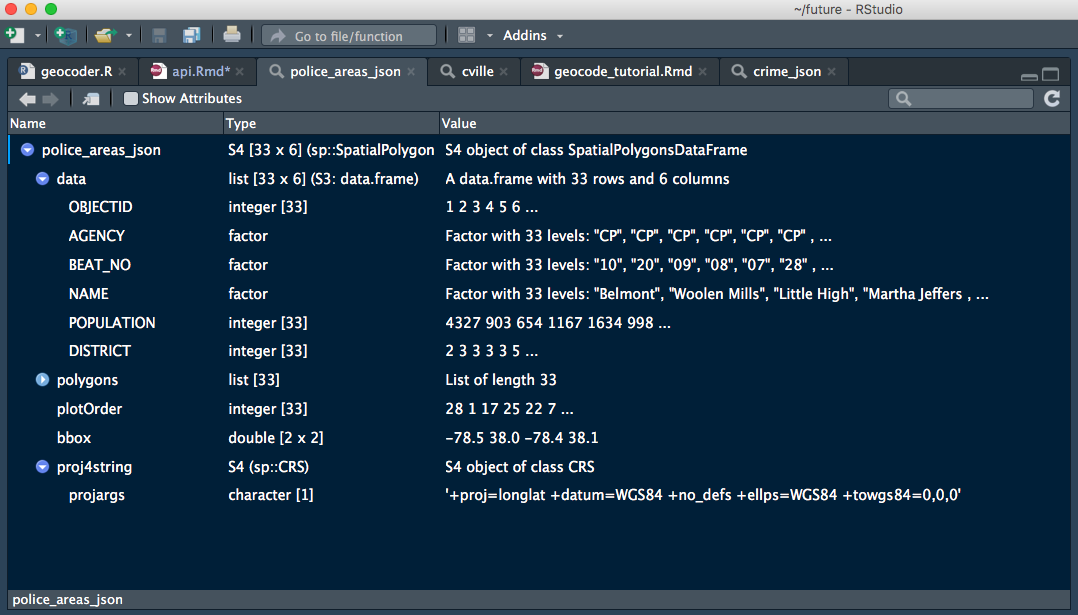
The data and polygons elements are the key components of a SpatialPolygonDataFrame. data is a list of information tables and polygons is list of sp::Polygons that contain the latitude and longitude cordinates necesary for mapping the region outlines. Indexing a SpatialPolygonDataFrame uses a special @ syntax to get to specific elements by name, so we would use police_areas_sp@data to look at just that section.

Notice both elements are the same length, Charlottesville is broken down into 33 police beats, so there is table information to accompany each map region. This means that a single SpatialPolygonDataFrame can be used to group the mapping information with accesory information, like population, crime rate, or real estate assesments.

head(police_areas_sp@data)

##   OBJECTID AGENCY BEAT_NO                 NAME POPULATION DISTRICT
## 0        1     CP      10              Belmont       4327        2
## 1        2     CP      20         Woolen Mills        903        3
## 2        3     CP      09          Little High        654        3
## 3        4     CP      08     Martha Jefferson       1167        3
## 4        5     CP      07       North Downtown       1634        3
## 5        6     CP      28 Charlottesville High        998        5

We could use a variety of map tools to plot a this type of SpatialPolygonDataFrame, including library(ggplot2), library(lattice) and library(mapview). Here we use library(leaflet) to plot the police beats and use the POPULATION data to color the regions. Leaflet is origially a JavaScript library for building interactive maps, which was ported to R and is pretty great, even ESRI (the ODP’s commercial partner) build a package with it.

library(leaflet) #v1.1.0
pal <- colorNumeric("viridis", NULL)

leaflet(police_areas_sp,
        options = leafletOptions(minZoom = 13, maxZoom = 15)) %>%
    addProviderTiles("OpenStreetMap.Mapnik") %>% # should look familiar
    addPolygons(color = "#a5a597", smoothFactor = 0.3, fillOpacity = .5,
                fillColor = ~pal(POPULATION),
                label = ~paste0(NAME, ": ", formatC(POPULATION, big.mark = ",")))

I’m not going to dive into the syntax of the leaflet code here, but the Leaflet for R website has great write ups for a variety of mapping options.